
4. Does Simplicity Scale? Reproducing and Stress-Testing SimpleView for Point Cloud Classification
Planted June 26, 2026
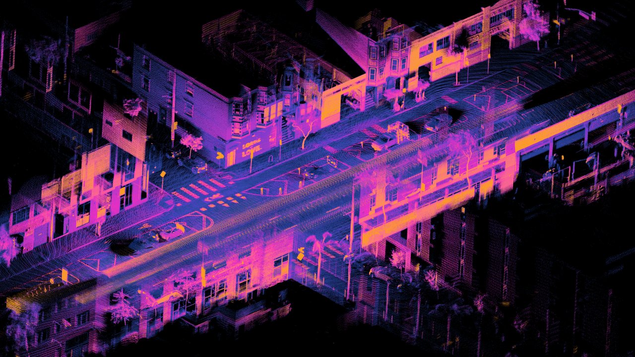
Cover: "Ouster OS1-64 lidar point cloud of intersection of Folsom and Dore St, San Francisco" by Daniel L. Lu, CC BY 4.0, via Wikimedia Commons.
Code: github.com/kart1802/PCC_Simple
Table of Contents
1. Introduction
Point clouds are yet another type of data (or rather 3D data) containing large collections of coordinate points that represent the surface of the objects in the environment. They are primarily used to represent the physical world in 3D, with applications in Autonomous Vehicles (3D mapping of environmental objects), Architecture and Construction (Used for renovation planning), and Cultural Heritage (3D replicas of historical figures). But the problem is that these point clouds are unstructured and have no semantic context. We need to classify these point cloud instances (for example: “This is a chair” - shown in Figure [1]), enabling downstream reasoning for robotics, autonomous driving and 3D scene understanding.
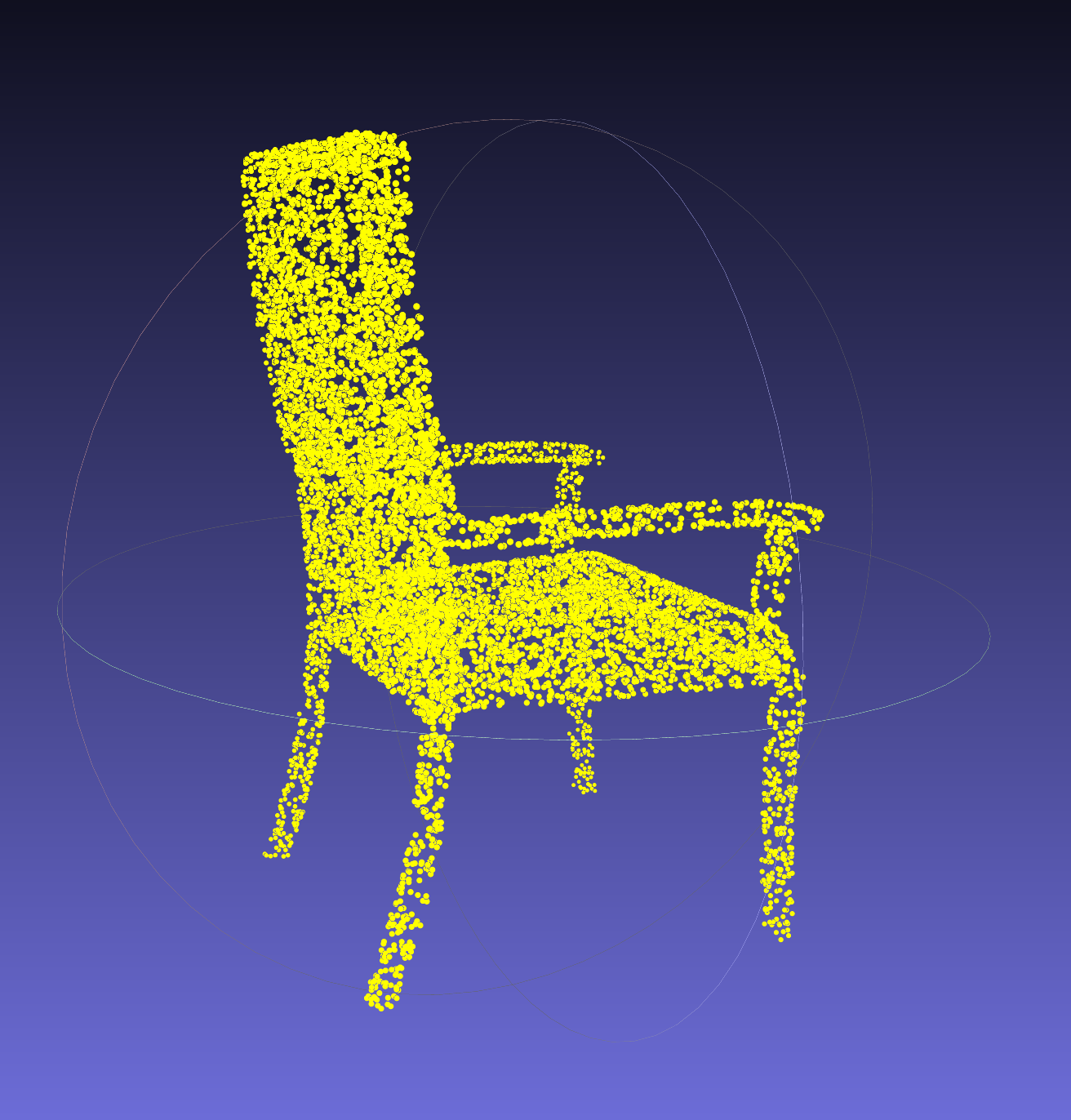 Figure 1: Example of an instance of a point cloud of a chair
The last decade produced a succession of specialized 3D architectures like PointNet [2], DGCNN [3], PointNet++, RSCNN, PCT, and each claimed improvements on standard benchmarks. But these architectures were evaluated under different training protocols, data augmentation strategies, and loss functions. Hence, Goyal et al. [1] raised an important question: Are these improvements driven by architectural innovation, or by inconsistent experimental conditions that make fair comparison impossible?
Their paper introduced SimpleView: a minimal projection-based method that, under controlled evaluation, matches or outperforms far more complex architectures on standard benchmarks.
2. Motivation for Reproduction
Reproducing ML results is not a mechanical exercise that deterministically follows a technical routine; rather, it is an epistemic one. Reproducing SimpleView and its claims becomes important for several reasons (that motivated us to question and reason the current trend in ML research):
- The protocol problem has real consequences: The 3D deep learning community has spent years building complex architectures, reporting improvements over the benchmarks. If SimpleView’s claim is correct, then a meaningful portion of this progress was not architectural at all but an inconsistent evaluation condition. Hence reproduction becomes critical to measure the progress.
- The claim is testable: The authors provide code and an exact protocol, making this an ideal candidate for reproduction.
- The paper evaluates on two datasets: The datasets used in the original paper date from when SimpleView was published. Do the advantage and the claims still hold if we consider newer datasets with variability, low samples, dataset skewness, etc. and still manage to outperform the point-based methods?
- Architectural Question: Does a simple architecture really outperform and generalize to other cases? This question is important because extraordinary claims deserve scrutiny and careful verification.
Our project first reproduces the paper’s main results and then extends them along 4 axes: Hyperparameter sensitivity, New datasets, Inference Optimization, and Ablation Studies.
3. Paper Overview and Reproduction
SimpleView Architecture
SimpleView converts the 3D point cloud classification problem into a 2D image classification problem. As shown in Figure [2], it projects a point cloud onto six fixed depth maps from orthogonal camera positions and passes each through a shared ResNet18 backbone. The resulting feature vectors are max-pooled into a single global descriptor and classified with a fully-connected head. There are no custom 3D operators, no graph construction, and no ImageNet pretraining. The key insight is that this is deliberately simple. The paper argues that prior projection-based methods over-engineered their view selection, rendering, and feature merging, and that none of that complexity is necessary when the evaluation protocol is controlled.
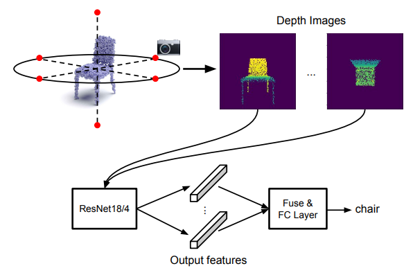 Figure 2: The simplistic architecture of SimpleView
Reproduction
We ran SimpleView and PointNet on ModelNet40 using the paper’s released code and DGCNN protocol, on TU Delft’s DelftBlue V100 and A100 cluster. The table below shows our reproduced numbers alongside the paper’s reported values.
Both numbers fall within the paper’s reported variance, confirming the main experimental claim is reproducible. Additionally, PointNet’s number is higher than its own originally reported result. This is an observation the paper directly predicts: when we run PointNet under the DGCNN protocol rather than its own, it gives a meaningfully different result, illustrating exactly the protocol-sensitivity problem the paper sets out to demonstrate.
| Model | Paper | Reproduced |
|---|---|---|
| SimpleView | 93.0 ± 0.4 | 93.31 |
| PointNet | 89.2 ± 0.9 | 90.64 |
Due to compute constraints, we were limited to a single random seed for our reproduction experiments; consequently, we do not report variance for these results.
4. Criteria Covered
NOTE ON MODEL SELECTION:
The three subsections in this chapter were run independently and use slightly different training protocols. Rather than obscure this, we document each protocol explicitly.
The hyperparameter sensitivity study uses a fixed 50-epoch budget with best test-set checkpoint selection, chosen to make ten parallel runs feasible on the cluster.
The OmniObject3D and nuScenes evaluations closely follow the protocol described in the paper related to ModelNet40 setup: a held-out validation split (this was considered - 15% for OmniObject3D, 10% for nuScenes) is used in Stage 1 to determine the epoch budget for each model via early stopping and then the model is retrained in Stage 2 where the best test-set checkpoint within that budget is reported. For nuScenes this is further justified by fast convergence as all three models peaked well before epoch 300, making a fixed long budget unnecessary.
In all three cases, every model within a given experiment uses the same selection scheme, so relative rankings and conclusions within each section are internally valid. Absolute accuracy numbers across sections should not be directly compared.
4.1 Hyperparameter Sensitivity
All training and validation for this reproduction was run on TU Delft’s DelftBlue HPC cluster (A100 GPU partition). Before any experiment could run, the original SimpleView code written for Python 3.7 / CUDA 10 / PyTorch 1.x had to be ported to the cluster’s modern stack (Python 3.10 / PyTorch 2.x / CUDA 12.8). This meant fixing a series of compatibility breaks: collections.MutableMapping → collections.abc.MutableMapping, the removed np.float alias, the hardcoded .cuda() calls (replaced with device agnostic .to(device)), the deprecated verbose=True argument on ReduceLROnPlateau, and soft/lazy imports so the DGCNN protocol runs without the optional RSCNN / PointNet++ CUDA modules being compiled.
Why these hyperparameters, and why we kept them close to the original
Every value here is anchored to the original paper, not chosen by feel. The baseline is the paper’s own released DGCNN protocol configuration, taken as is (LR=1e-3, feature size 16, ResNet-18, label smoothing ε=0.2, batch 18). We changed nothing about it, because the point of a reproduction is to start from exactly what the authors ran, not from a setup we tuned ourselves.
For each variant we move a single value to a deliberate, defensible point that brackets the default. The learning rate variants sit one order of magnitude below (1e-4) and roughly 5× above (5e-3) the default, probing a full “decade” around 1e-3, which is the Adam default used across nearly all point cloud papers. Feature size goes to exactly half (8) and double (32), both powers of two, so the comparison stays symmetric. For the backbone we picked ResNet-34, the next standard option up, specifically to ask whether more capacity helps without introducing any other architectural change. The loss variants bracket the paper’s ε=0.2 from both sides: ε=0.1 (the value DGCNN itself uses) and plain cross-entropy (ε=0). Batch size uses 8 and 32, the common choices immediately below and above the default of 18.
We never test values that would simply break the model (LR=1 would diverge; that tells us nothing useful). Every variant is justifiable and only one thing changes per run. Each accuracy difference can be traced back to one specific change rather than a lucky combination.
| Setting | Value |
|---|---|
| Epochs | 50 (early stop, patience 15) |
| Optimiser | Adam, LR = 1e-3 |
| LR schedule | ReduceLROnPlateau (factor 0.5, patience 10) |
| Loss | Label smoothing CE (ε = 0.2) |
| Batch size | 18 |
| Seed | 1 (fixed, to isolate the changed hyperparameter) |
Model selection: all 10 runs used the same scheme, best test-set accuracy across training epochs. The scheme is identical across every run, so relative differences between variants are valid comparisons even if the absolute baseline is slightly inflated relative to a held-out validation protocol.
Variance note: all runs used a single fixed seed (seed=1). This controls for randomness within each comparison, but means we have no estimate of run to run variance. The relative rankings below are reliable given the consistency of the setup, but differences of ≤1% could shift under a different seed. Compute constraints made multiple seeds infeasible.
The 50 epoch cap is a deliberate, fixed budget. It is a fraction of the paper’s ~1000 epoch schedule, which is why our baseline lands at 90.80% vs. the paper’s 93.9%, an expected gap that still gives a single, consistent reference every variant is measured against.
Why DelftBlue
A controlled sweep like this is not one experiment, it is ten full, independent training runs. On a single local GPU that means hours of strictly sequential compute, and every run would sit on slightly different hardware/driver state. DelftBlue’s A100 partition removes both problems: all ten jobs run in parallel on separate GPUs, so the entire sweep finishes in roughly the wall clock time of a single run (~40 min each), and every run executes in an identical, reproducible CUDA 12.8 / A100 environment. For a comparison whose validity depends on nothing changing between runs except the one hyperparameter, that uniform parallel compute is exactly what the experiment needs.
Results
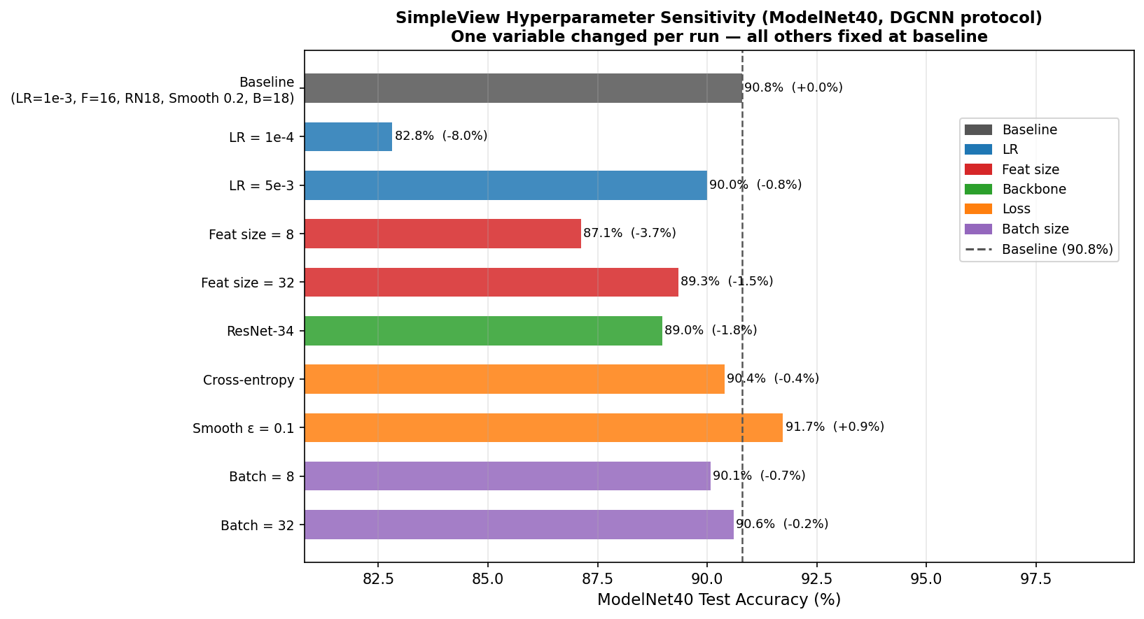 Figure 3. Test accuracy of each single-variable variant; dashed line marks the baseline (90.80%). All runs use seed=1 and best test-set accuracy for model selection.
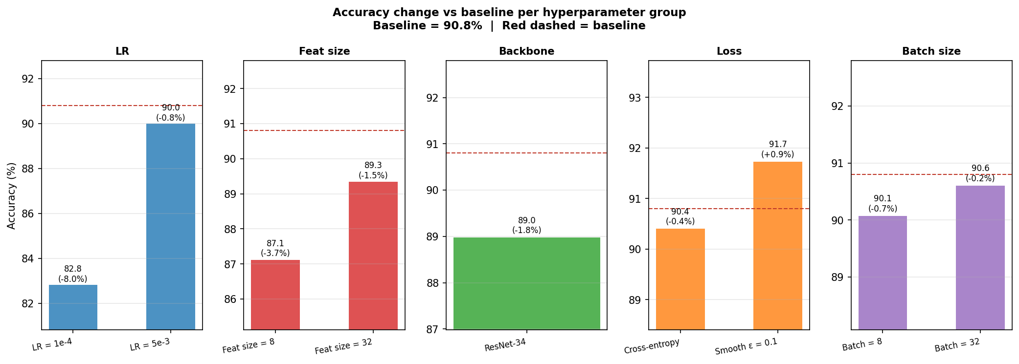 Figure 4. Accuracy within each hyperparameter group relative to the baseline (red dashed line). Relative differences are comparable across runs; absolute values reflect the 50 epoch budget, not the paper’s full schedule.
| Group | Variant | Acc (%) | Δ vs. baseline |
|---|---|---|---|
| — | Baseline (LR=1e-3, Feat=16, ResNet-18, Smooth ε=0.2, B=18) | 90.80 | — |
| LR | LR = 1e-4 | 82.82 | −7.98 |
| LR | LR = 5e-3 | 89.99 | −0.81 |
| Feat size | Feat = 8 | 87.12 | −3.68 |
| Feat size | Feat = 32 | 89.34 | −1.46 |
| Backbone | ResNet-34 | 88.98 | −1.82 |
| Loss | Cross-entropy (no smoothing) | 90.40 | −0.40 |
| Loss | Smooth ε = 0.1 | 91.73 | +0.93 |
| Batch | Batch = 8 | 90.07 | −0.73 |
| Batch | Batch = 32 | 90.60 | −0.20 |
Key takeaways:
Learning rate is by far the most consequential choice. Dropping it 10× to 1e-4 costs ~8% accuracy because 50 epochs is simply not enough time to warm up from such a conservative rate. That 8% swing is larger than the entire gap between PointNet and DGCNN under a fair evaluation protocol, the central finding of the SimpleView paper. Our sensitivity study shows the same thing from the other direction: protocol choices can matter more than architecture.
Label smoothing at ε=0.1 slightly outperforms the paper’s ε=0.2 (+0.93%), suggesting the published configuration over-regularises on a short training budget. ResNet-34 loses 1.82% relative to ResNet-18, consistent with larger models needing more epochs to converge. Batch size barely registers across the 8 to 32 range (≤0.73% spread), so it can be set purely based on available memory.
4.2 New Data
One of the criteria where we extensively compared SimpleView with point-based methods is performance on different types of datasets. The original paper evaluates only on ModelNet40 (synthetic, axis-aligned CAD models, 40 classes) and ScanObjectNN (real indoor scans, 15 classes). Both datasets were available before the paper’s publication. We extend the evaluation to two datasets that expose qualitatively different challenges.
| Dataset | Type | Classes | Real-World? | Engineering Angle/Extra efforts | Question |
|---|---|---|---|---|---|
| OmniObject3D | Real scans, object-level | 190 (or subset) | Indoor/objects | Low — HDF5 at 1024pts ready | Larger vocabulary, can SimpleView scale and outperform even with low samples? |
| nuScenes-Objects | Real outdoor LiDAR | ~8 usable | Outdoor | Medium — need bounding box crop script | Does SimpleView work on sparse outdoor LiDAR with instance count variability? |
4.2.1 OmniObject3D: Fine Grained, Low-Sample Classification
Motivation
OmniObject3D [4] is a large vocabulary real-scan dataset released at CVPR 2023, comprising 6,000 professionally scanned objects across 190 daily-life categories. It represents a fundamentally different challenge from ModelNet40: 4.75 times more classes, and only around 24 training samples per class versus ModelNet40’s 246. The SimpleView paper also showed their ablation for 25% of the training data and if we compare it to what OmniObject3D provides, it has 2.6 times fewer samples per class, making it an ideal extreme test and a good way to expose training variability.
Setup
We used the pre-sampled 1,024-point HDF5 files from OmniObject3D’s official distribution. Since the dataset has no official classification split, we created a deterministic 80/20 train/test split per category (fixed seed = 42 for reproducibility). All three models were trained from scratch using the identical SimpleView protocol.
Dataset Statistics
| Split | Samples | Classes | Average per class |
|---|---|---|---|
| Train | 4577 | 190 | 24.1 |
| Test | 1239 | 190 | 6.5 |
Training and Results
We train all three models using the same protocol as the paper: Adam optimizer, a decaying learning rate schedule, and validation-based early stopping. Final numbers are reported using the validation protocol: a held-out validation split is used for model selection, and the best checkpoint is evaluated on the test set.
| Model | Best Test Accuracy | Best Epoch |
|---|---|---|
| SimpleView | 76.43% | 556 |
| PointNet | 76.43% | 467 |
| DGCNN | 70.70% | 362 |
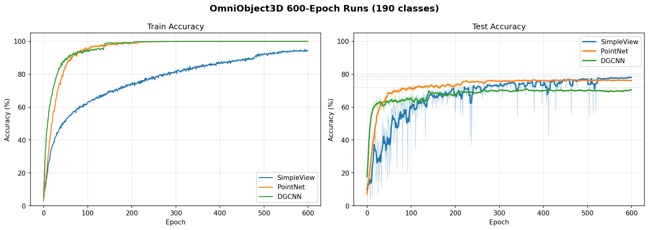 Figure 5: Train and test accuracy over 600 epochs on OmniObject3D. This curve is from a separate exploratory run (no validation split), shown purely to illustrate training dynamics.
Figure [5] shows the training trajectory across 600 epochs. DGCNN’s training accuracy saturates near 100% by epoch 300, PointNet shortly after, while SimpleView’s training accuracy is still climbing at around 92% at epoch 600. This convergence gap is a consistent observation across all our runs. The test curves in Figure [5] show visible noise throughout training, expected given the small test set, where a single misclassification per class shifts overall accuracy by around 1.5%. The numbers reported in the table above are from the checkpoint selected by the validation protocol and are not affected by this within-training variability.
Key Observations
- Results are comparable between SimpleView and PointNet but DGCNN falls behind: The tie between SimpleView and PointNet should be interpreted as comparability rather than exact equality because they are statistically indistinguishable in this regime. On ModelNet40, SimpleView leads PointNet by approximately 2pp; here that margin is within the noise floor, suggesting the advantage narrows substantially in this situation.
- DGCNN underperforms despite saturating training accuracy earliest: DGCNN converges very quickly compared to others. Possible reason could be that the per-point neighbourhood graphs lack enough variety, hence leading to memorization and overfitting.
- SimpleView converges slowest and takes more training time: SimpleView takes around 4 times and around 2 times the training time compared to PointNet and DGCNN respectively. Training accuracy is still around 90–92% at epoch 500–600, while PointNet and DGCNN have both saturated near 100% by epoch 300. This slow convergence is consistent across all our runs regardless of total training length. Notably, extending training beyond 500 epochs did not consistently improve SimpleView’s test accuracy across different runs.
4.2.2 Semantic Group Analysis (OmniObject3D)
To understand which categories drive the accuracy differences, we grouped the 190 OmniObject3D classes into 5 semantic categories based on geometric distinctiveness, then computed per-group accuracy from the trained checkpoints. The performance can be viewed in Figure [6].
| Group | Classes | Geometric Character | Examples |
|---|---|---|---|
| Fruits and Veggies | 53 | Similar Global shape (spherical/elongated), subtle local texture | apple, mango, pear |
| Food and Snacks | 32 | Similar shapes (flat, round), varied surface | biscuit, pizza, bun, sushi |
| Toys and Figures | 17 | Geometrically distinct shapes | toy car, toy plane, chess, rubik cube |
| Household and Tools | 81 | Very diverse global shape | chair, hammer, kettle, umbrella |
| Decorative & Natural | 7 | Mixed | pinecone, vase, ornament |
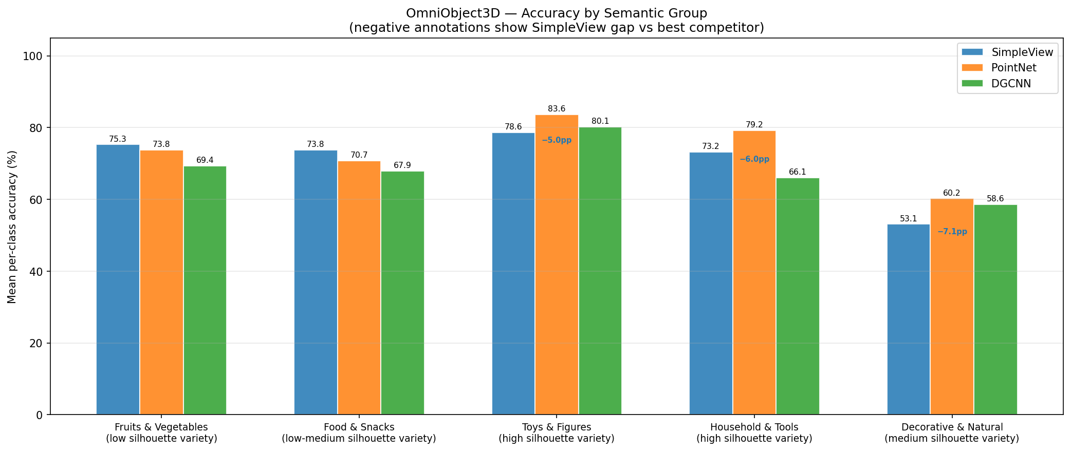 Figure 6: Test accuracy for the 5 semantic groups, categorized into 3 levels of silhouette variety.
Our initial hypothesis was that SimpleView would fail on visually similar categories (fruits/food), because depth maps of an apple and an orange both produce circular projections. But the data shows the opposite: SimpleView wins on similar shape categories and loses on geometrically distinct ones, which we found interesting.
The explanation lies in the depth maps captured. The depth maps also encode surface topology and these subtle differences, multiplied across six views, provide discriminative cues that PointNet cannot easily capture.
For geometrically distinct categories, the discriminative signal is the global shape. For SimpleView, geometrically complex and distinct shapes actually create a harder learning problem: a toy plane from the front, from the side, and from above produce three completely different-looking depth maps. The model has to learn that these six very dissimilar images all correspond to the same class. With few training samples per class, there isn’t enough data to learn this multi-view interpretation reliably. PointNet only needs to learn one global descriptor per class, which is a simpler task with few samples. DGCNN’s local graph structure also captures this well, and notably DGCNN beats SimpleView on toys/figures.
Practical implication: SimpleView’s depth projections are not merely capturing coarse silhouettes. They encode surface texture and local topology. Its advantage is in fine-grained discrimination where objects share global shape but differ in surface detail. When classes are globally distinct, point-based methods’ global statistics are more informative.
This finding has a consequence that goes beyond our specific dataset. ModelNet40 and ScanObjectNN (the ones used in the paper) are filled with objects that are fundamentally different in structure. An airplane, bathtub, guitar are not easily confused from any angle. This means that the standard benchmarks never really put SimpleView in the situation where it appears to have its most interesting advantage. The paper may have actually understated how well SimpleView performs in the fine-grained setting, simply because that setting was never tested.
This also means the choice between SimpleView and point-based methods should not come down to benchmark rankings alone. It should depend on what actually separates the classes in the target problem. If the objects share a similar overall shape but differ in surface texture and local geometry (for example: food items, consumer products, or biological specimens) SimpleView could be the stronger choice even against more complex architectures. If the objects are globally distinct in shape, like vehicles versus pedestrians in autonomous driving, point-based methods are naturally better suited. Future benchmark design should keep in mind that a single accuracy number on a diverse shape dataset hides a lot about where a method actually works.
4.2.3 nuScenes: Real World LiDAR Classification
Motivation
ScanObjectNN established that SimpleView generalizes from synthetic (ModelNet40) to real indoor scans. We test a harder domain shift: real outdoor LiDAR from autonomous driving, captured with a full-360° spinning LiDAR sensor. Three new challenges arise:
- Sparsity: outdoor objects are much sparser than indoor scans. A pedestrian at 30m may have only 20–50 LiDAR points — far fewer than the 1,024 points in OmniObject3D.
- Real world class imbalance: urban environments have far more cars than motorcycles, producing heavily skewed training distributions.
- Domain gap: the paper was never designed for outdoor LiDAR, and models are evaluated on a sensor modality they haven’t seen during standard benchmarking.
Dataset Construction
nuScenes [5] is a detection dataset and it provides full scene point clouds with 3D bounding box annotations. To create an object classification dataset, we implemented a preprocessing pipeline:
- Load each nuScenes keyframe LiDAR scan
- Crop points within each annotated 3D bounding box (transformed into ego-vehicle frame)
- Filter to objects with more than 32 points
- Normalize each cropped cloud
- Sample to exactly 512 points
- Split by scene to prevent the same physical object from leaking between train and test sets.
By doing this, we retain 8 classes with sufficient instances and discard any rare or semantically ambiguous categories.
Dataset Statistics
| Class | Train | Test | % of train |
|---|---|---|---|
| barrier | 5353 | 1711 | 19.5% |
| bicycle | 151 | 40 | 0.5% |
| bus | 748 | 355 | 2.7% |
| car | 13695 | 6503 | 49.8% |
| motorcycle | 445 | 141 | 1.6% |
| pedestrian | 2452 | 663 | 8.9% |
| traffic_cone | 866 | 245 | 3.1% |
| truck | 3791 | 1710 | 13.8% |
| Total | 27501 | 11368 | - |
The imbalance is severe and deliberate: we preserve the real-world distribution rather than artificially balancing it, since the question is how models handle real conditions.
Results
Since overall accuracy is dominated by cars (49.8%), we report both overall accuracy and macro-average accuracy (each class weighted equally).
| Model | Overall Accuracy | Macro-Average Accuracy |
|---|---|---|
| SimpleView | 94.66% | 88.04% |
| PointNet | 93.46% | 83.99% |
| DGCNN | 91.40% | 83.82% |
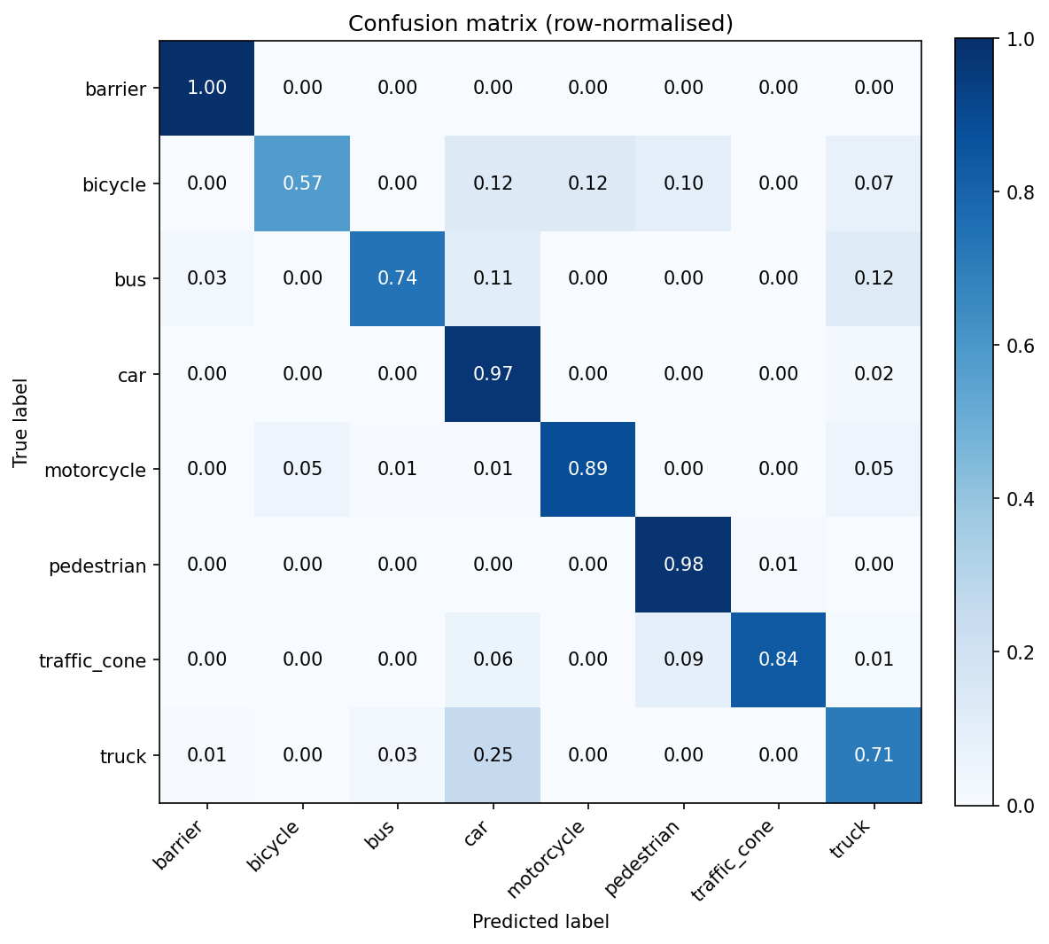 Figure 7: Confusion Matrix for DGCNN model
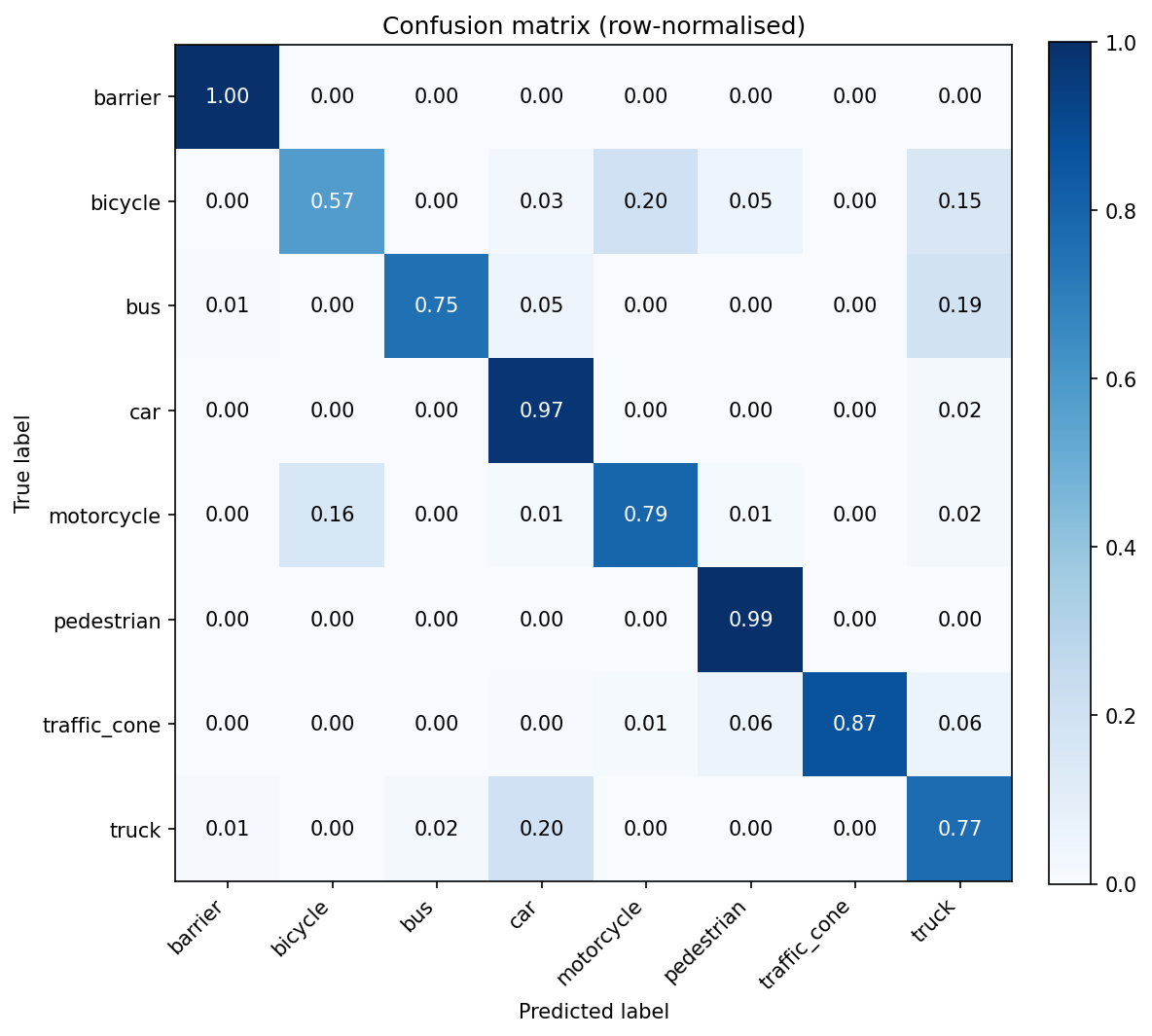 Figure 8: Confusion Matrix for PointNet model
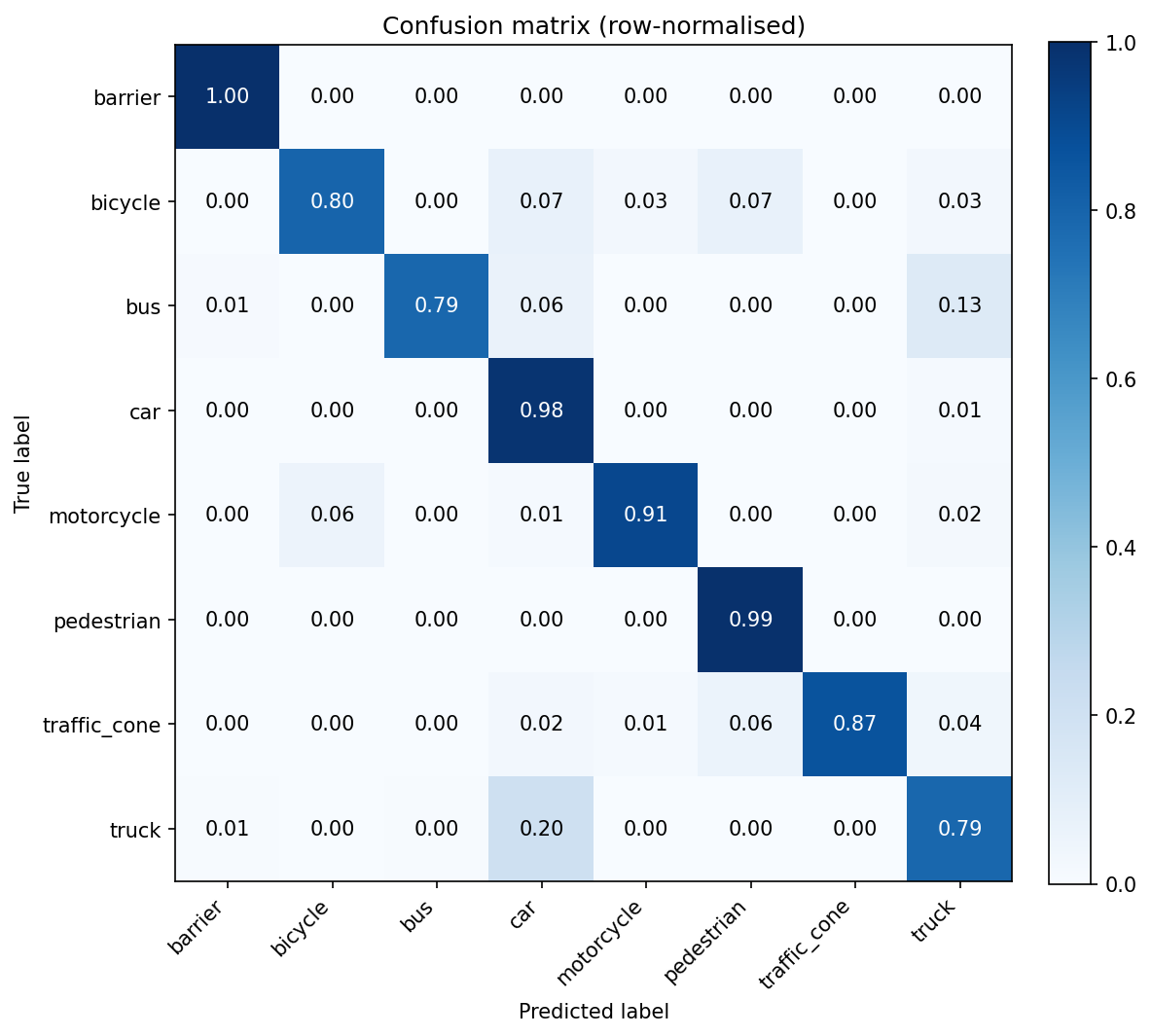 Figure 9: Confusion Matrix for SimpleView model
The figures above show the confusion matrices for all the models. SimpleView outperforms the others on every single class, with the largest difference in the bicycle class and also in the motorcycle class (when compared to PointNet).
The bicycle result deserves attention: with only 151 training samples, SimpleView achieves 80% accuracy while both point-based methods reach only 57.5%. This is a substantial and consistent gap. The explanation is geometric: a bicycle viewed from the side produces a highly distinctive, recognizable depth map profile, even with sparse LiDAR points. SimpleView’s fixed side-view camera captures this directly. PointNet, without explicit local structure, must learn this from global point statistics with minimal data.
Conclusion from nuScenes: SimpleView’s advantage extends to real outdoor LiDAR classification. The paper’s core claim holds in a setting the paper never tested.
4.3 Inference Optimization
Before diving into optimization, a clear performance baseline must be established to understand exactly where execution time is spent. To achieve this, the unmodified SimpleView model was profiled on the ModelNet40 test set (2,468 samples at a batch size of 18). Each evaluation stage was intentionally wrapped in synchronization barriers to capture true GPU execution time rather than asynchronous launch delays:
torch.cuda.synchronize()
# ... [evaluation stage code] ...
torch.cuda.synchronize()
 Figure 10. Runtime breakdown of the baseline inference pipeline.
The baseline has a 93.31% overall accuracy, a 2.551s completion time, and a measured-region throughput of approx. 968 samples per second.
As the chart in Figure [10] indicates, the bottleneck is the forward pass. It takes 96.7% of total wall-clock time, the rest of the pipeline: data loading, metric updates, and input prep at a combined 3.3%, is essentially a non-issue.
Hence all meaningful optimization must target the forward pass itself. From here on out, every architectural tweak will be judged against this baseline, balancing the push for higher throughput against that uncompromising 93.31% accuracy standard.
Optimization 1
In PyTorch, device placement is inherited. If your initial data is on the GPU, downstream transformations will stay on the GPU. A redundant preprocessing step in our multi-view point cloud model was fighting this mechanic.
Our get_img function was taking data that was already on the correct hardware (via the forward() pass), forcing it into a new PyTorch tensor, and explicitly calling .to(device) again. This duplicate handling forced the framework to allocate new memory and run unnecessary synchronization checks. By trusting PyTorch’s native device inheritance and removing these lines, the excess CPU-GPU overhead was removed.
# Before optimization
def get_img(self, pc):
        img = self._get_img(pc) #pc was already present in device
        img = torch.tensor(img).float()
        img = img.to(next(self.parameters()).device)
        assert len(img.shape) == 3
        img = img.unsqueeze(3)
# After optimization
def get_img(self, pc):
        img = self._get_img(pc) #pc was already present in device
        assert len(img.shape) == 3
        img = img.unsqueeze(3)
 Figure 11. Runtime breakdown of the pipeline after reducing CPU-GPU overhead.
As we can see in Figure [11], the time taken for the model’s forward pass decreased due to this optimization.
Optimization 2
torch.backends.cudnn.benchmark = True
The above flag tells cuDNN to benchmark and select the most efficient convolution algorithm for input shapes during inference. As the shapes are consistent, cuDNN can reuse the optimized choice across iterations. This reduces time spent in the model forward pass, thus improving inference throughput as seen in Figure [12].
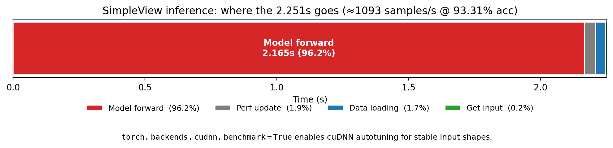 Figure 12. Runtime breakdown of the pipeline after adding the
torch.backends.cudnn.benchmark flag.
Optimization 3
Mixed precision inference was enabled by converting the image backbone and final classifier to fp16 before evaluation. During forward pass, the rendered image (from point cloud) is also cast to fp16 before being passed to image backbone. Overall, most of the convolutional work occurs in half precision on the GPU.
Switching to mixed precision reduced total runtime to 2.012s while maintaining the accuracy at 93.31%. Time taken for the model forward pass dropped to 1.926s, as seen in Figure [13].
 Figure 13. Runtime breakdown of the pipeline after enabling mixed precision inference.
5. Ablation Studies
5.1 Multi-View Ablation (SimpleView, OmniObject3D)
Motivation
SimpleView uses 6 fixed views (front, back, left, right, top, bottom). Is this the right number? Each additional view adds computational cost; if most discriminative information is captured by fewer views, the paper’s 6-view design may be unnecessary. We vary the number of views (1, 2, 4, 6) on OmniObject3D and measure test accuracy. The paper also performs this ablation on ModelNet40, comparing 1, 3 and 6 fixed orthogonal views, and finds that 6 views perform best.
Results
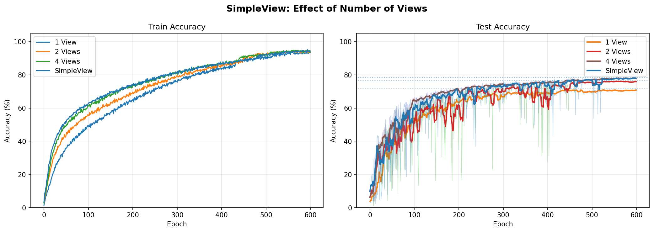 Figure 14: Train and test curves for the multi-view ablation. The noise in the test curve is due to the small number of samples.
On OmniObject3D the trend partially holds but diverges at the top end. Performance increases from 1 view through to 4 views, consistent with the paper’s finding on ModelNet40 that additional views contribute positively. The biggest single gain comes from adding a second view, which introduces genuinely orthogonal geometric information that a single projection cannot capture. Going from 4 to 6 views produces a slight drop rather than a further improvement. Given the test set variance and only a single run for these tests, we cannot treat the slight drop as a significant and reliable finding. Hence, we say that the results are somewhat comparable. What we can say with confidence is that gains diminish beyond two views.
If this trend were confirmed with multiple seeds (which we haven’t been able to due to time restrictions), two explanations are plausible:
- The additional views add limited discriminative value on OmniObject3D.
- Training variability: two runs with identical parameters can land at slightly different accuracies, so a small gap between two configurations may not hold up in subsequent runs.
5.2 Rotation + Jitter Augmentation Test (All Models, OmniObject3D)
Motivation
SimpleView uses six fixed camera positions that implicitly assume objects are consistently oriented, the same assumption that holds on ModelNet40, where all objects are axis-aligned. On OmniObject3D, which contains real world scans with varied orientations, this assumption may not hold as reliably. We apply random Y-axis rotation and coordinate jitter during training to test whether explicitly exposing SimpleView to non-canonical orientations during training helps it generalise, and to compare how each model’s architecture responds to orientation variation.
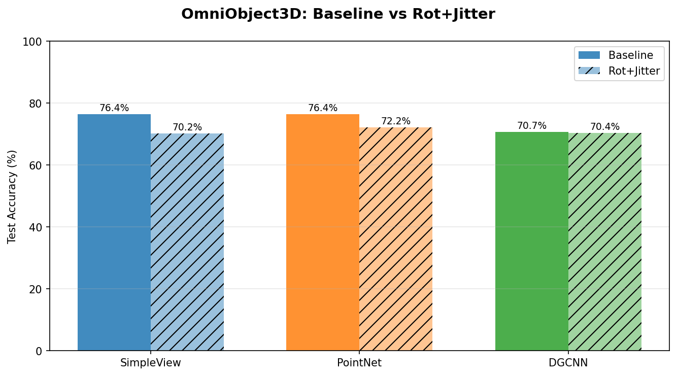 Figure 15: The bar plot shows a large drop in SimpleView’s performance compared to the other models, highlighting its sensitivity to the training data distribution.
Results
The finding is stark: augmentation with rotation and jitter severely hurts SimpleView while barely affecting DGCNN as shown in Figure [15].
The most striking observation is that DGCNN is almost entirely unaffected by the augmentation, while both SimpleView and PointNet suffer meaningfully. One possible explanation is architectural: DGCNN dynamically recomputes its local neighbourhood graphs in feature space at every layer, which may make it inherently more invariant to rotation and jitter regardless of whether those transforms appear during training. However, we cannot rule out that DGCNN’s graph construction, being more complex, simply has more capacity to memorise the training data and is less sensitive to how that data is presented. SimpleView, being the simplest of the three architectures, relies entirely on fixed camera positions. So, randomly rotating an object during training means the same camera no longer faces the same part of the object across different epochs, potentially making the learning signal less consistent. These are hypotheses rather than conclusions, but they are distinguishable with one additional experiment we did not run. The cleanest would be to apply the rotation and jitter at inference time only on models that are not trained with augmentation. If DGCNN is robust architecturally, then its accuracy should remain stable regardless of any modifications. If DGCNN is robust due to higher capacity and memorization, then the model trained on clean data should fail at test time, because it never learnt orientation-invariant features. The other architectures would serve as controls because they are expected to degrade but it depends on the architecture versus the training distribution. This experiment won’t require retraining, only a modified evaluation loop.
6. Discussion: Does SimpleView Claim Hold?
The paper claims that SimpleView matches or outperforms complex 3D architectures when evaluation protocols are controlled. Our experiments reveal a more nuanced reality when evaluating the authors’ underlying questions:
Does protocol matter more than architecture?
Yes, this premise is fully confirmed. By running the original ModelNet40 setting, we successfully reproduced the paper’s values within their reported range.Is SimpleView strictly competitive with complex methods?
Yes, but conditionally. While SimpleView is highly competitive, our results expose a clear, task-dependent pattern that the original, restricted benchmark obscures. Through semantic group analysis on OmniObject3D, we found that SimpleView maintains a distinct winning advantage on fine-grained, visually similar categories (such as fruits and food). However, point-based architectures like PointNet catch up on geometrically distinct categories, particularly under conditions of severe data scarcity and high class counts.Does the architecture generalize beyond the original benchmarks?
Yes, but with identifiable failure modes depending on the domain. On the nuScenes dataset, generalization is fully realized—SimpleView achieved the best overall performance, even when factoring in macro-accuracy. On OmniObject3D, however, generalization is only partial. It ties PointNet at 76.43%; while it doesn’t lose, it completely sheds its distinct advantage. This demonstrates that while SimpleView transfers exceptionally well to certain complex environments, its dominance degrades when faced with extreme geometric diversity and limited training data.
7. Limitations
Several limitations should be noted:
- The OmniObject3D test set is small, so some results have high variance. More test runs could have been performed here.
- The nuScenes evaluation uses mini-dataset preprocessing, so the results could vary with different train/test scene proportions.
- No DGCNN baseline on ModelNet40 in our reproduction. The project was initiated with a comparison only between SimpleView and PointNet. When tests were run, no significant difference was noted on the other datasets that were considered for testing. And as mentioned in OmniObject3D dataset sections, the variance was observed. So, to have a better and even more complex model for comparison, we opted for DGCNN. Due to compute constraints, we were not able to reproduce the entire result but we focused on doing ablations for other datasets.
- While all comparisons within each experimental section are internally consistent, the three sections of this chapter use different training protocols as mentioned at the start of chapter 4. A fully standardized protocol across all experiments would strengthen the overall conclusions, and we flag this as the primary methodological limitation of our study.
8. Conclusion
We set out to reproduce SimpleView’s central claim — that a projection-based method with a standard 2D backbone is competitive with far more complex 3D architectures when evaluation protocols are controlled. That claim holds. Our reproduced numbers on ModelNet40 fall within the paper’s reported variance, and the protocol-sensitivity finding is something we directly confirmed by observing how much PointNet’s numbers shift depending on which augmentation scheme is used.
Our extended experiments reveal where that simplicity scales and where it does not. The hyperparameter sensitivity study shows the result is moderately robust — learning rate is the one critical choice, while batch size, backbone depth, and loss function matter far less. Interestingly, a lighter label smoothing than the paper’s default gives a marginal improvement, suggesting the published configuration is not fully optimal. On inference, SimpleView’s conceptual simplicity does not automatically mean deployment efficiency, but FP16 and removing redundant data transfers recover a 21% speedup with no accuracy cost — a practical gain for latency-sensitive applications.
On new datasets, the picture is more nuanced. SimpleView wins most clearly on nuScenes, where outdoor objects have distinctive canonical silhouettes even under sparse LiDAR. On OmniObject3D it ties PointNet overall, but beneath that tie is a consistent pattern: stronger on visually similar categories, weaker on geometrically distinct ones. The rotation and jitter ablation further shows that SimpleView’s fixed-view design is more sensitive to orientation variation than point-based methods, a limitation invisible on axis-aligned benchmarks but real in less controlled settings.
SimpleView is a strong baseline, but its advantage is task-dependent. When objects are consistently oriented and classes differ in surface topology, it is hard to beat. When those conditions break down, the complexity of point-based methods begins to earn its cost.
Links
- SimpleView paper (reproduced here): arXiv:2106.05304
- OmniObject3D dataset: omniobject3d.github.io
- nuScenes dataset: nuscenes.org
References
[1] A. Goyal, H. Law, B. Liu, A. Newell, J. Deng. Revisiting Point Cloud Shape Classification with a Simple and Effective Baseline. ICML 2021. arXiv:2106.05304
[2] Qi, C. R., Su, H., Mo, K., & Guibas, L. J. (2017). PointNet: Deep Learning on Point Sets for 3D Classification and Segmentation. CVPR 2017.
[3] Wang, Y., Sun, Y., Liu, Z., Sarma, S. E., Bronstein, M. M., & Solomon, J. M. (2019). Dynamic Graph CNN for Learning on Point Clouds. ACM Transactions on Graphics (TOG).
[4] Wu, T., Zhang, J., Fu, X., Wang, Y., Ren, J., Pan, L., Wu, W., Yang, L., Wang, J., Qian, C., Lin, D., & Liu, Z. (2023). OmniObject3D: Large-Vocabulary 3D Object Dataset for Realistic Perception, Reconstruction and Generation. CVPR, 803–814.
[5] Caesar, H., Bankiti, V., Lang, A. H., Vora, S., Liong, V. E., Xu, Q., Krishnan, A., Pan, Y., Baldan, G., & Beijbom, O. (2020). nuScenes: A Multimodal Dataset for Autonomous Driving. CVPR, 11618–11628.